Controller Design for a Differential-Drive Robot
A one-month research internship on linear control for autonomous ground robots. I modelled a differential-drive robot, wrote PID and LQR controllers in Python, and ran them on the Quanser QBot hardware to track parabolic, sinusoidal and free-form paths. At the end I formulated an MPC controller for constrained motion and explored first ideas in nonlinear control.
The QBot Platform is an open-architecture ground robot on a differential-drive base: two driven wheels, one on each side. My first task was to learn the hardware and to send velocity commands to it from Python.
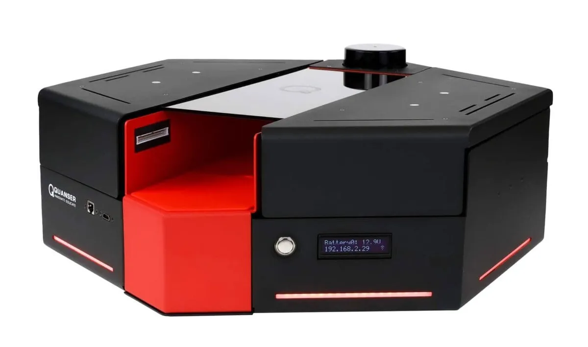
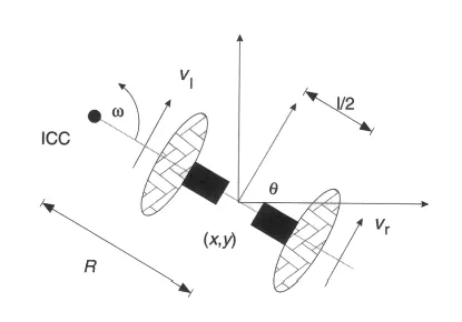
I wrote the forward and inverse kinematics. The wheel speeds give the robot's linear speed v = (vR + vL)/2 and turn rate ω = (vR − vL)/L. Odometry integrates ẋ = v cos θ, ẏ = v sin θ, θ̇ = ω at each time step. Angle normalisation keeps θ in range, so the heading does not drift.
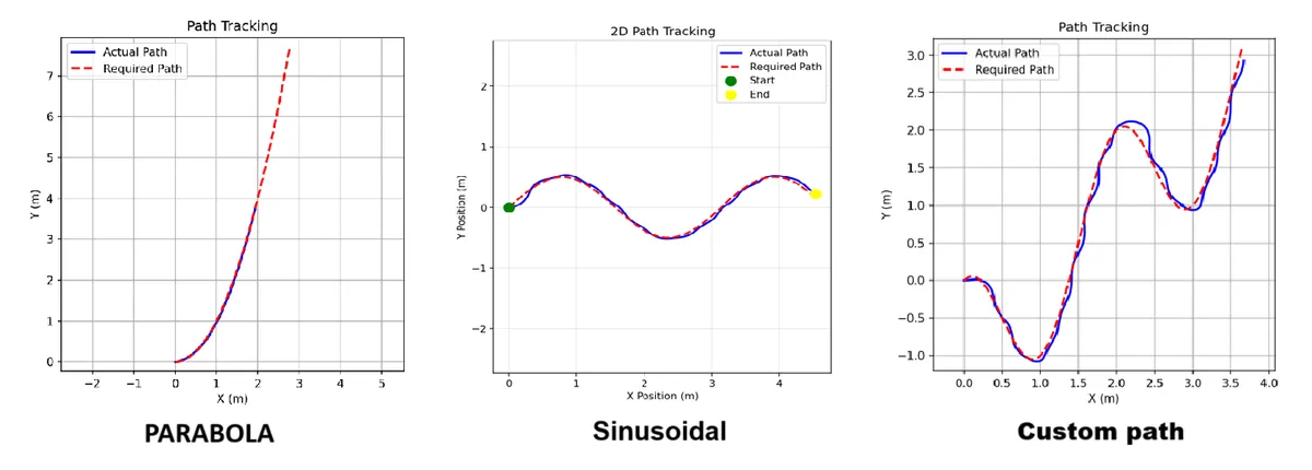
I wrote one PID controller for position and one for heading. Their outputs are velocity commands in the world frame. The code transforms them into the robot frame and limits them for safety. After several rounds of debugging the command structure and tuning the gains on the hardware, the robot tracked parabolic, sinusoidal and free-form paths closely.
I linearised the model around a nominal forward speed v0 and a small heading angle (cos θ ≈ 1, sin θ ≈ θ). This gives ẋ = Ax + Bu, with state [x, y, θ] and input [v, ω]. SciPy's continuous algebraic Riccati solver gives P, and the gain is K = R−1BTP. The control law is u = −K(x − xref), with velocity saturation for the real robot. I tuned the weights Q (tracking error) and R (control effort). LQR did better than PID, mainly in dynamic conditions.
In the last part I formulated model predictive control: over a horizon of N steps, minimise the tracking error and control effort, subject to the linear model and limits on states and inputs, then apply only the first input (receding horizon). The plan was a quadratic-programming solver with velocity and acceleration limits. This part was a start for constrained motion planning, not a finished result.
My part
I did all of the work on this page: the kinematic model, the PID and LQR code, the hardware tests and the tuning.
Challenges
- Wheel slip: slip made the odometry wrong over time, so the estimated pose moved away from the real pose.
- Command structure: PID outputs are in the world frame, but the robot takes commands in its own frame. It took several iterations to get the transform and the limits right.
- Tuning on hardware: gains that worked in simulation needed changes on the real robot.
What I learnt
- Differential-drive kinematics and odometry, from equations to working code.
- Controller design from start to end: model, design, implementation and tuning.
- How to linearise a nonlinear model, set up LQR and solve the Riccati equation.
- How to move a controller from theory to a real robot.
I thank Dr. Shyam Kamal for his supervision and Mrs. Priyanka for her guidance during the internship.